Skip to content

A server can finish a computation efficiently and still contribute to an inefficient site. The result depends on what happens after electrical power reaches the processor, how the cooling system captures its heat, how pumps and heat exchangers move that energy, and whether the mechanical plant can reject or reuse it without creating additional demand. Each component can perform exactly as designed while the complete system delivers less useful computing work than its individual specifications suggest. System-level accounting becomes more difficult when server, coolant distribution, refrigeration, electrical conversion, and heat rejection measurements use different boundaries, sampling intervals, or reporting systems. Thermal chain efficiency therefore begins with a question that component-level testing cannot answer: how much useful, reliable computing work does the entire site deliver for the electrical and thermal resources it consumes?

The answer requires a different way of following energy through digital infrastructure. Power enters through an electrical connection, passes through conversion stages, and reaches equipment that turns electricity into computation and heat. Cooling equipment then circulates fluid, transfers heat across interfaces, and moves the remaining thermal load toward rejection or recovery. Each handoff establishes operating conditions for the next component, and an upstream change can improve or worsen downstream performance depending on the system design and operating point. Changes in server power can alter coolant return conditions, while higher coolant supply temperatures may reduce refrigeration demand when equipment limits permit and may change the temperature available to a heat recovery system. These relationships make thermal performance inseparable from electrical distribution, workload behavior, control logic, and the physical boundary at which the site receives power and delivers useful work.
Why a Perfect Component Can Still Build an Inefficient System
An engineering acceptance test can confirm that a server, cooling distribution unit, or chiller meets its intended performance requirements without proving that the complete site operates efficiently. Each test isolates a particular function, establishes controlled conditions, and determines whether the equipment performs within its expected operating envelope. Component tests may not reproduce all interactions that occur when computing demand changes, coolant temperatures shift, electrical losses accumulate, and control systems respond to competing requirements. A server may complete its assigned work with less electrical demand, yet the surrounding infrastructure may consume additional power to maintain coolant flow, preserve thermal stability, or reject heat at an unfavorable temperature. The equipment has delivered its local improvement, but the site has not necessarily converted that improvement into a comparable reduction in total energy demand.
The component performs, but the site tells a different story
The underlying issue begins with the way electrical energy moves through computing infrastructure and becomes heat. Electricity passes through distribution and conversion equipment before reaching processors, memory, networking hardware, and other electrical loads. The computing equipment uses that electricity to execute instructions, move data, maintain internal states, and support communication between components, while much of the electrical energy ultimately becomes heat that the cooling system must manage. That heat does not travel automatically from its source to a useful destination, because the cooling architecture must establish fluid movement, maintain pressure, transfer energy across heat exchangers, and preserve suitable operating conditions. Every stage introduces constraints that influence the performance of the stages around it, including temperature differences, pressure losses, conversion overhead, and control responses.

This is why a favorable component specification cannot serve as a reliable substitute for integrated operating evidence. A pump with efficient electrical characteristics can still move fluid through a poorly balanced circuit, while a high-performance heat exchanger can operate within a system that supplies it with unsuitable flow or temperature conditions. A chiller can meet its rated performance under its test conditions but consume more electricity when the wider installation requires a lower leaving-water temperature or faces an unfavorable heat rejection environment. Similar problems arise when server-level power improvements encourage operators to increase workload density without checking whether the cooling plant can maintain the required operating envelope. These interactions do not make component specifications irrelevant, because they provide essential inputs for equipment selection, design validation, and troubleshooting.
Why moving data and removing heat belong in the same calculation
Computing performance depends on more than the processor’s ability to execute instructions with limited electrical demand. Modern workloads move information between memory, accelerators, storage, and networking components, and those transfers consume energy while creating heat across the system. The physical placement of data, the frequency of communication, the amount of synchronization required, and the relationship between processing stages all influence the electrical demand associated with useful work. A processor can complete an individual operation efficiently while the wider application spends additional time and energy moving information between components or waiting for dependent tasks to finish. The resulting heat then enters a cooling system whose response depends on where the electrical loads sit, how their thermal output changes, and how effectively the installation transfers that heat toward rejection.
The relationship becomes especially important when a workload changes its operating pattern. A system may alternate between intensive processing, data movement, synchronization, and periods of lower activity, producing a thermal profile that differs from its average electrical demand. Cooling controls that respond slowly can continue circulating fluid or maintaining operating conditions that no longer match the current load, while aggressive control changes can create instability or compromise equipment requirements. An apparently efficient server configuration may also shift heat concentration toward particular racks or coolant branches, increasing local flow requirements even when total computing demand remains stable. Those effects can change pump demand, heat exchanger performance, and the operating point of the wider cooling plant without producing an obvious warning in a server-only report.
The Interface Tax That Never Shows Up on the Spec Sheet
The interface between two efficient components can introduce losses that neither component’s individual performance report fully captures. Heat must cross a physical boundary between the server’s internal cooling arrangement and the facility’s coolant circuit, and that transfer depends on the temperatures, flow rates, pressure conditions, and thermal resistance present at the interface. A heat exchanger cannot transfer energy without a temperature difference, and the required difference depends on its design, operating conditions, and the properties of the fluids involved. When a heat exchanger requires a larger temperature approach, engineers should assess whether the connected circuits can maintain the required thermal transfer without changing supply temperatures, flow conditions, or supporting equipment demand. Each response changes the energy requirements elsewhere in the chain, even when the heat exchanger itself remains within its specified operating range.
Every handoff changes the conditions for the next component
Coolant distribution illustrates how these losses accumulate across connected equipment. Fluid must travel through pipes, valves, manifolds, filters, and heat exchangers before returning to the equipment that requires cooling, and every restriction contributes to the pressure conditions that pumps must overcome. Poor circuit balancing can direct excessive flow through one branch while leaving another branch with insufficient flow for its thermal demand. Engineers may respond by increasing pump speed, raising differential pressure, or changing valve positions, but those adjustments can increase electrical consumption or move other branches away from their intended operating points. A pump can consequently demonstrate efficient operation at its own measurement boundary while the complete distribution circuit consumes more energy than necessary to deliver the required cooling. Measuring pump input alongside circuit pressure, branch flow, coolant temperatures, and server demand reveals whether the distribution system delivers the required thermal service without unnecessary hydraulic overhead.
Electrical conversion introduces a related interface problem because power reaches the computing equipment through interconnected distribution stages. Transformers, power conversion equipment, uninterruptible power systems, and rack-level power supplies each operate within their own efficiency envelope, which changes with loading and operating conditions. Electrical conversion losses generally become heat within the equipment or its surroundings; reducing those losses can lower cooling demand when the eliminated heat would otherwise have entered the site’s cooling load. However, a component-level report may not capture how its operating point interacts with the rest of the distribution system or how a change in electrical load affects supporting equipment. A complete assessment follows power from the site intake through the relevant distribution stages and into the computing load, while separately accounting for cooling and other supporting demand.
Why the mechanical plant pays for upstream decisions
The chiller and heat rejection system inherit the conditions established by the equipment and coolant circuits upstream. A design that requires unusually cold coolant can force the refrigeration system to operate under a less favorable temperature lift, while a restrictive circuit can increase pumping demand before the heat reaches the chiller. Heat rejection equipment must then release that energy into the surrounding environment, with its performance influenced by ambient conditions, fluid temperatures, airflow, and control settings. These requirements interact because changing the temperature at one point can reduce demand in one part of the plant while increasing it elsewhere. Raising a coolant supply temperature may reduce refrigeration demand, for example, but the benefit depends on whether the servers and intermediate heat exchangers can still meet their thermal requirements.
The interface tax also becomes difficult to identify when different teams control different parts of the system. Computing engineers may optimize server power and workload placement, mechanical engineers may adjust coolant temperatures and pump operation, and electrical teams may manage distribution losses and capacity constraints. Each group can improve its own equipment while leaving the wider operating conditions unchanged or inadvertently making them less favorable. If server and chiller monitoring do not share synchronized records or relevant operating data, their individual reports may show a change in electrical demand without establishing the upstream conditions that contributed to it. Separate dashboards compound the problem when they use different sampling intervals, equipment labels, measurement boundaries, or definitions of normal operation. Connecting those records around a shared timeline allows engineers to determine whether a change in one subsystem produced a corresponding improvement or penalty elsewhere in the chain.
Return Temperature as a System Efficiency Signal
The temperature of coolant returning from computing equipment provides information about how the system transports heat, but its meaning depends on the conditions under which the equipment operates. Supply temperature establishes the thermal conditions entering the cooling circuit, while return temperature reflects the combined effects of equipment heat transfer, coolant flow, workload distribution, and the behavior of the surrounding circuit. The difference between these temperatures helps engineers interpret the heat carried by the fluid when they combine it with mass flow and the fluid’s thermal properties. A warmer return does not automatically indicate better efficiency, just as a cooler return does not automatically indicate better cooling performance. Low flow can produce a large temperature difference while leaving some equipment inadequately cooled, whereas high flow can reduce the temperature difference while increasing pump demand.
Reading the heat that leaves the rack
The physical relationship follows the heat carried by a moving fluid, which depends on its mass flow, specific heat capacity, and temperature change across the equipment. Engineers can estimate the transferred thermal power by combining those properties, provided they account for the actual fluid mixture and use consistent measurement units. This calculation connects a temperature reading to the heat transported through the circuit, rather than treating the reading as an efficiency score on its own. A return-temperature increase may reflect greater computing demand, reduced coolant flow, a change in workload placement, or a change in the thermal behavior of the equipment. Engineers must therefore compare the reading with corresponding electrical input and workload records before deciding whether the change represents improved heat capture or a developing cooling constraint.
A return-temperature profile can also reveal how evenly the installation distributes cooling across its computing loads. When similar equipment operates under comparable conditions, persistent differences between branches may indicate unequal flow, inconsistent thermal contact, variations in workload, or differences in local heat exchanger performance. Those differences matter because a shared supply temperature does not guarantee that every rack receives the same effective cooling conditions. A control system that reacts only to an aggregate temperature can conceal a local constraint until the affected equipment approaches its operating limit. Branch-level temperature and flow measurements help engineers separate genuine differences in thermal demand from problems in the distribution circuit. Linking these readings to workload placement and equipment status allows the site to respond to the actual source of a thermal imbalance instead of compensating for it by increasing cooling across the entire installation.
Heat quality determines whether recovery has practical value
Capturing heat and making that heat useful are separate engineering tasks. The thermal energy leaving computing equipment may carry substantial heat content, yet its temperature can limit the applications that can accept it directly. A receiving process may require a higher temperature than the cooling circuit can provide, which means a heat pump or another temperature-lifting arrangement may need to increase the heat’s usefulness. That equipment consumes electricity, and the additional energy demand changes the net value of the recovery arrangement. Engineers should therefore evaluate the temperature available at the recovery boundary, the temperature required by the receiving process, the stability of the heat supply, and the energy needed to bridge any gap between them.
Heat quality also depends on the difference between the temperature at which energy becomes available and the temperature at which another process can use it. Thermodynamic limits constrain how much useful work a system can extract from heat, and those limits become more restrictive when the heat source sits close to the surrounding environmental temperature. A large quantity of low-temperature heat can consequently have less direct practical value than a smaller quantity delivered at a temperature that matches a receiving process. This does not make low-temperature heat worthless, because appropriately designed systems can use it for suitable heating demands or combine it with heat pumps. It means that recovery assessments must consider temperature, timing, demand, and conversion requirements instead of reporting captured heat as though every unit had the same practical value.
The Blind Spot Between Rack Inlet and Facility Outlet
The thermal chain depends on information moving between systems that were often designed to control different parts of the installation. Server firmware and hardware management mechanisms can adjust operating states in response to temperature, power limits, and other device-specific constraints, while workload software determines how computing tasks use the available resources. Runtime software schedules workloads and manages the available computing resources, while the building management system coordinates mechanical equipment, coolant temperatures, pumps, and other plant functions. Each system can make a locally appropriate decision without understanding the consequences for the complete installation. A runtime may place additional work on a server because its computing resources appear available, while the cooling controls respond only after the resulting thermal load reaches their sensors.
Why separate control systems lose the operating picture
The problem extends beyond delayed responses because each control layer may describe the same operating condition differently. Firmware can report processor temperature, power limits, and throttling events, while workload software records job progress, resource utilization, and application performance. The mechanical control system may report coolant supply and return temperatures, pump states, valve positions, and chiller demand, while electrical monitoring records power at different points in the distribution chain. These records become difficult to reconcile when timestamps differ, equipment identifiers do not match, or one system reports an average while another records a brief event. An engineer may see an increase in cooling demand without being able to connect it to the workload that triggered the change. Establishing shared equipment identifiers, synchronized timestamps, consistent units, and documented measurement boundaries provides the foundation for investigating those interactions.
Telemetry also needs to distinguish a component’s available capacity from the capacity that the complete system can safely deliver. A server may have spare processing capacity while its rack approaches a coolant flow constraint, or a cooling plant may have available capacity while electrical distribution limits prevent the computing load from increasing. Those conditions produce different operating decisions, even when a conventional utilization dashboard presents similar signals. A useful control architecture combines computing demand, electrical headroom, thermal conditions, and equipment constraints to determine which resources can accept additional work. Such coordination does not require every control system to surrender its independent protective functions, because local safeguards must remain capable of responding to unsafe conditions. Instead, the architecture needs a shared view of the constraints that determine whether additional computing work can run without compromising service requirements or increasing total site demand disproportionately.
Why an efficiency gain must survive operational constraints
A measured efficiency improvement can disappear when the system encounters a power cap, thermal limit, or workload performance requirement. A processor may use less energy for a particular operating state, but the application may take longer to complete if the system reduces clock speed or limits available computing resources. The lower instantaneous power demand does not establish a genuine improvement unless the assessment also accounts for the completed work and the time required to deliver it. Similar effects can emerge when thermal controls restrict workload placement to protect a heavily loaded rack or when electrical limits prevent the installation from using otherwise available computing capacity. Engineers should therefore connect power and temperature telemetry with application-level performance records, including completion time and service-level objective compliance.
Commissioning provides the opportunity to verify whether these controls work together before operators rely on them during normal service. Engineers can introduce controlled workload changes, observe how the computing and cooling systems respond, and confirm whether electrical and thermal measurements capture the resulting changes at the relevant boundaries. They can also test what happens when a sensor becomes unavailable, a pump changes operating state, a cooling branch loses capacity, or the workload reaches a protective limit. These tests should establish which controller has authority during conflicting conditions and how the system returns to normal operation after an event. The resulting evidence gives operators a practical basis for deciding whether the controls can sustain an efficiency improvement without creating a reliability problem. An efficiency claim that cannot survive those operating conditions remains an unverified design expectation rather than a demonstrated property of the installed system.
How One Unmeasured Handoff Erases Two Measured Wins
Efficiency calculations become misleading when teams combine improvements measured at different boundaries without checking how those boundaries interact. A server-level improvement describes the relationship between computing output and the electrical power measured at the server, while a cooling improvement describes a different relationship between thermal demand and supporting electrical consumption. The two results cannot establish the site’s overall improvement unless engineers account for the workload, operating conditions, and energy flows that connect them. A change in server performance can alter the heat load entering the cooling system, while a change in coolant temperature can alter the electrical demand required to remove that heat. The resulting system performance depends on the combined behavior of the components, not the arithmetic sum of their individual efficiency claims. A reliable assessment therefore reconciles all relevant measurements against a common operating period and a consistent site boundary.
Why separate efficiency gains cannot simply be added together
Consider a server configuration that reduces its electrical demand for a defined workload while the cooling plant experiences an unfavorable change in operating conditions. If the change requires colder coolant, additional pumping, or greater refrigeration effort, the cooling system may consume more electricity than it did before the server improvement. The site could consequently retain some of the server-level benefit while losing a portion of it through the supporting infrastructure. Engineers cannot determine the net effect from the server report alone, because that report does not include the additional energy consumed downstream. They must compare the total electrical input before and after the intervention while confirming that the workload delivered equivalent useful output. The comparison should record relevant temperature, flow, and environmental conditions to help identify possible causes of changes in overall performance, with controlled testing used where necessary to establish causation.
The same reasoning applies when teams evaluate heat exchanger performance independently from the chiller and distribution system. A heat exchanger can maintain the required thermal transfer while operating with a larger temperature difference than the wider system would ideally require. That condition may force the upstream circuit to deliver colder fluid or cause the downstream plant to work harder to meet its temperature target. The heat exchanger’s local performance report may still show successful operation, yet the additional temperature requirement can increase energy consumption elsewhere in the installation. Engineers should therefore evaluate the interface against the temperature conditions required by both connected circuits and the electrical consequences of maintaining those conditions. This method identifies whether an apparently acceptable component operating point creates a penalty that the separate equipment reports fail to reveal.
Building a measurement chain that survives scrutiny
A defensible end-to-end calculation begins with a clear statement of the boundary and the useful output being measured. The electrical boundary should identify the relevant incoming power and the supporting loads included in the calculation, while the workload boundary should specify which completed computing tasks count as useful output. Engineers then need measurements that connect those boundaries, including server power, distribution losses where measurable, cooling equipment demand, coolant temperatures, and relevant flow conditions. All records should use compatible timestamps and comparable operating periods so that transient changes do not create artificial differences between the baseline and the intervention. The team should also document sensor accuracy, missing readings, estimation methods, and any equipment excluded from the calculation. These controls make the resulting comparison reproducible and prevent the apparent improvement from depending on an undocumented change in measurement scope.
The measurement chain should also separate direct observations from calculated estimates. Electrical meters can establish energy consumption at defined points, while temperature and flow sensors can support calculations of heat transported through a coolant circuit. Those calculations depend on the fluid properties, sensor placement, calibration, and assumptions used to represent the operating conditions. Engineers should avoid presenting an estimated thermal transfer value as though a meter measured it directly, particularly when uncertainty in flow or temperature measurements could materially change the result. A consistent measurement plan should identify which quantities the site measures directly, which quantities it calculates, and how uncertainty affects the comparison. This transparency allows operators to determine whether an apparent improvement exceeds measurement uncertainty or merely reflects the limitations of the monitoring arrangement.
When Useful Work Becomes the Only Metric That Survives Contact With Reality
The purpose of computing infrastructure is to deliver useful work within the operating conditions that the application requires. Electrical efficiency matters because power has physical, operational, and financial consequences, but lower consumption alone cannot establish that a computing system performs better. A configuration that uses less electricity while completing fewer tasks, taking longer to respond, or missing required service levels may reduce instantaneous demand without improving the service the site delivers. Thermal chain efficiency must therefore connect energy consumption with a clearly defined workload output and the conditions required to deliver it. The appropriate output measure depends on the application, because a completed simulation, a processed transaction, and an inference request do not represent interchangeable units of work. A useful assessment identifies the relevant output first and then determines how much electrical and thermal support the site requires to produce it reliably.
Measuring output that the site can actually deliver
For AI inference, useful output may involve completed requests, generated tokens that meet application requirements, or another workload-specific measure that reflects the service actually delivered. The measurement must account for response quality and latency requirements, because a system that generates output faster but fails to meet the required quality standard has not necessarily delivered more useful work. For interactive inference workloads, time to first token and response latency can be relevant performance measures, while total completion time and throughput may be more appropriate for longer-running or batch workloads, depending on the application’s service requirements. Batch workloads may prioritize completion throughput, whereas interactive workloads may place greater weight on predictable response times and tail latency. Engineers should select the measure that matches the application rather than assuming that a single computing metric represents every workload.
The available electrical capacity must account for the limits that actually constrain computing deployment, including power distribution, cooling capability, equipment protection, and the operating margin needed for reliable service. A site may have unused electrical capacity but lack sufficient cooling capacity at the required supply temperature, or it may have adequate cooling equipment but face a constraint in its electrical distribution path. The relevant denominator therefore cannot rely on the site’s theoretical grid connection alone if the complete installation cannot safely deliver that capacity to productive computing equipment. Engineers should define deployable capacity using verified operating limits and report the assumptions that determine how much capacity remains available for useful work. This approach connects computing productivity with the infrastructure that supports it instead of treating the electrical connection as though it were equivalent to usable computing capacity.
Why workload-aware thermal efficiency matters
Workload-aware measurement changes how engineers interpret cooling improvements because the same thermal arrangement can support different levels of useful output. A higher coolant supply temperature may reduce refrigeration demand, but its value depends on whether the computing equipment can sustain the required workload without thermal throttling or service degradation. A lower pump setting may reduce electrical consumption, but the resulting flow conditions must still maintain adequate heat transfer across every relevant branch. Engineers should evaluate these changes under representative workloads and compare the useful output, total electrical demand, coolant conditions, and service performance across equivalent operating periods. They should also observe how the system responds when workloads shift, because an operating point that performs well during a stable test may behave differently under changing demand.
An effective optimization process consequently needs to connect application software, server controls, coolant management, and plant operation through a shared definition of success. The workload layer identifies the service that the site must deliver, while the computing layer records the resources and electrical power required to complete it. Thermal and electrical controls then report whether the infrastructure can sustain that workload within the available operating envelope. Engineers can use those records to test alternative workload placements, temperature targets, and cooling strategies without confusing a reduction in demand with an improvement in productive output. They should retain the original service requirements throughout the comparison and reject apparent gains that depend on missed targets or unacceptable operating risks. Thermal chain efficiency becomes meaningful when the complete site delivers more qualifying work from its available resources while maintaining the thermal, electrical, and reliability conditions that the service requires.
Start From the Boundary You Have, Then Work Inward
A reliable thermal design begins with the conditions under which the site must deliver computing work, rather than with an isolated component’s efficiency target. Engineers should establish the available electrical supply, the capacity of the distribution system, the thermal conditions the computing equipment can accept, and the cooling capacity that the installed plant can sustain. They should also account for the commissioning schedule, the physical space available for equipment, the operating environment, and any realistic opportunity to supply recovered heat to another process. These requirements define the conditions that the complete installation must satisfy before individual components can be selected or optimized. Starting from this boundary makes it easier to identify incompatible assumptions, such as a server design that requires coolant conditions the selected mechanical plant cannot maintain efficiently.
Design around the site’s actual operating limits
The next step is to work inward through the electrical, computing, distribution, and thermal systems while preserving the relationships established at the boundary. Electrical engineers can characterize the power available to computing equipment, mechanical engineers can establish the coolant conditions required to transport heat, and computing engineers can determine the workload performance that the installation must sustain. Each discipline then evaluates its component choices against the requirements imposed by the connected systems. A change to one design assumption should trigger a review of the interfaces it affects, including electrical demand, coolant flow, temperature requirements, control responses, and heat rejection capacity. This process helps prevent an improvement in one subsystem from creating an avoidable constraint in another. It also gives commissioning teams a consistent basis for verifying that the completed installation performs according to the integrated design rather than merely passing separate equipment acceptance tests.
Commissioning should verify the operating relationships that the design depends on, not simply confirm that individual components start and run. Teams should test representative workloads, record electrical demand at defined boundaries, observe coolant temperatures and flow conditions, and establish how the cooling plant responds when computing demand changes. They should verify that the control systems exchange the information needed to manage constraints and that protective actions do not create unexpected consequences elsewhere in the installation. Where the design includes heat recovery, commissioning should establish whether the receiving process can accept the available thermal energy under its actual operating conditions. The team should retain a baseline that links useful computing output with electrical consumption, cooling demand, and the conditions under which the measurements occurred.
Make end-to-end verification part of normal operation
The work does not end when commissioning confirms that the installation meets its initial performance requirements. Computing workloads change, equipment ages, control settings evolve, and maintenance activities can alter the operating conditions that originally supported the site’s efficiency. Operators therefore need a continuing measurement process that connects workload performance, electrical demand, coolant conditions, and mechanical plant operation. When the site changes a server configuration, adjusts a coolant temperature, modifies pump controls, or introduces a new workload, the assessment should establish whether the intervention improved the complete system under comparable conditions. Engineers should also review measurement quality, because a failed sensor or an inconsistent reporting boundary can create an apparent improvement without changing the physical performance of the installation.
The central engineering task is to preserve efficiency as energy moves from the site’s electrical boundary through computing equipment and into the systems that transport, reject, or recover heat. A component improvement matters when the complete installation can retain that benefit without compromising workload performance, cooling requirements, or reliable operation. They also expose the interfaces where temperature differences, hydraulic resistance, control delays, and conversion losses can weaken the results that individual component reports appear to demonstrate. Starting from the site boundary and working inward gives designers, commissioning teams, and operators a common method for identifying those losses and verifying the effect of corrective action. Thermal chain efficiency is ultimately a property of the connected system, demonstrated by the useful work the site delivers and the total resources required to sustain it.